
1. はじめに
本記事では、Fortran の高速シミュレーション能力と Python の機械学習ライブラリを効果的に組み合わせ、高精度な合金強度予測モデルを構築した過程と結果について詳しく説明します。この手法により、材料設計プロセスの効率化を目指しました。
1.1 Fortran を使用した理由
- 数値計算に特化した言語であり、大規模シミュレーションに適している
- 高速な実行速度により、大量のシミュレーションデータを効率的に生成できる
1.2 Python を使用した理由
- 豊富な機械学習ライブラリ(scikit-learn 等)が利用可能
- データ処理や可視化のためのツールが充実している
- 柔軟性が高く、モデルの試行錯誤が容易
2. Fortran によるシミュレーション
2.1 シミュレーションの概要
Fortran を用いて、3元系合金の組成と温度に基づく強度計算シミュレーションを実装しました。以下の要素を考慮しています:
- 3つの元素の組成比(ランダムに生成)
- 温度範囲(300K〜1300K、ランダムに設定)
- 合金強度の計算(物理モデルに基づく)
- 熱伝導率の計算(組成と温度に依存)
2.2 シミュレーションコードの詳細
モジュール: alloy_properties
このモジュールでは、合金の強度と熱伝導率を計算する関数を定義しています。
module alloy_properties
  implicit none
  real, parameter :: k_boltzmann = 1.380649e-23 ! ボルツマン定数

contains
  function calculate_strength(composition, temperature)
    real, dimension(:), intent(in) :: composition
    real, intent(in) :: temperature
    real :: calculate_strength, solid_solution_strength, precipitation_strength
    real :: base_strength, temperature_factor

    ! 基本強度(合金組成による)
    base_strength = sum(composition * [5.0, 7.0, 9.0])
    ! 固溶強化(単純化モデル)
    solid_solution_strength = 2.0 * (abs(composition(1) - composition(2)) + abs(composition(2) - composition(3)))

    ! 析出強化(温度依存)
    temperature_factor = exp(-(temperature - 300) / 300) + 0.1 * sin(temperature / 100)
    precipitation_strength = 3.0 * sum(composition**2) * temperature_factor

    ! 全体の強度 (GPa)
    calculate_strength = base_strength + solid_solution_strength + precipitation_strength

    ! 1-10 GPaの範囲に収める
    calculate_strength = max(1.0, min(10.0, calculate_strength))
  end function calculate_strength

  function calculate_thermal_conductivity(composition, temperature)
    ! ... (熱伝導率計算のコード)
  end function calculate_thermal_conductivity
end module alloy_properties
メインプログラム: alloy_simulator
このプログラムでは、10,000 回のシミュレーションを実行し、結果を CSV ファイルに出力します。
program alloy_simulator
  use alloy_properties
  implicit none
  integer, parameter :: num_elements = 3, num_simulations = 10000
  real, dimension(num_elements) :: composition
  real :: temperature, strength, thermal_conductivity
  integer :: i

  open(unit=10, file='alloy_results.csv', status='replace')
  write(10,'(A)') 'Comp1,Comp2,Comp3,Temperature,Strength,ThermalConductivity'

  do i = 1, num_simulations
    call random_number(composition)
    composition = composition / sum(composition) ! 組成の正規化
    call random_number(temperature)
    temperature = temperature * 1000 + 300 ! 300K to 1300K

    strength = calculate_strength(composition, temperature)
    thermal_conductivity = calculate_thermal_conductivity(composition, temperature)

    write(10,'(3(F10.6,","),F12.6,",",ES16.6,",",F12.6)') &
          composition(1), composition(2), composition(3), &
          temperature, strength, thermal_conductivity
  end do

  close(10)
  print *, 'Simulation completed. Results saved in alloy_results.csv'
end program alloy_simulator
2.3 シミュレーション結果
10,000 回のシミュレーションを高速に実行し、以下の形式の CSV ファイルを生成しました:
Comp1,Comp2,Comp3,Temperature,Strength,ThermalConductivity
0.367024,0.194390,0.438586,1197.792969,7.970929E+00,277.878418
0.527210,0.398865,0.073926,653.494141,7.441678E+00,233.700012
...
3. Python による機械学習モデルの構築
3.1 データの前処理とモデル構築
Python の scikit-learn ライブラリを使用して、ランダムフォレスト回帰モデルを構築しました。以下のコードで、データの読み込み、前処理、モデルの構築を行いました。
def load_and_preprocess_data(file_path):
    data = pd.read_csv(file_path)
    X = data[['Comp1', 'Comp2', 'Comp3', 'Temperature']].copy()
    y = data['Strength']
    # 新しい特徴量の追加
    X['Temperature_squared'] = X['Temperature'] ** 2
    X['Temperature_log'] = np.log(X['Temperature'])
    X['Comp1_Comp2'] = X['Comp1'] * X['Comp2']
    X['Comp2_Comp3'] = X['Comp2'] * X['Comp3']
    X['Comp1_Comp3'] = X['Comp1'] * X['Comp3']
    return X, y

def train_and_evaluate_model(X, y):
    X_train, X_test, y_train, y_test = train_test_split(X, y, test_size=0.2, random_state=42)

    model = RandomForestRegressor(n_estimators=100, random_state=42)
    model.fit(X_train, y_train)

    y_pred = model.predict(X_test)

    mse = mean_squared_error(y_test, y_pred)
    r2 = r2_score(y_test, y_pred)

    return model, X_test, y_test, y_pred, mse, r2
3.2 結果
モデルの性能
Mean Squared Error: 0.002132075173628251
R2 Score: 0.9972610356820358
構築したモデルは、テストデータに対して高い予測精度を示しました。
特徴量の重要度
Comp1: 0.0854570968886335
Comp2: 0.19478767561775534
Comp3: 0.030206712048394143
Temperature: 0.03575820604012142
Temperature_squared: 0.036926865036260186
Temperature_log: 0.03825979626421548
Comp1_Comp2: 0.5577227177502317
Comp2_Comp3: 0.0016841758596077671
Comp1_Comp3: 0.019196754494780376
特徴量の重要度分析から、以下の点が明らかになりました:
Comp1_Comp2(元素1と2の相互作用)が最も重要な特徴量で、全体の約55.8%を占めています。Comp2(元素2の組成比)が次に重要で、約19.5%の寄与があります。- 温度関連の特徴量はそれぞれ3-4%程度の重要度を示しています。
3.3 視覚化
予測 vs 実際の値のプロットと特徴量重要度のバープロットを作成しました。これらのグラフから、モデルの予測精度の高さと各特徴量の相対的な重要度を視覚的に確認できました。
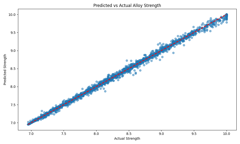
予測 vs 実際の値のプロット
特徴量重要度のバープロット
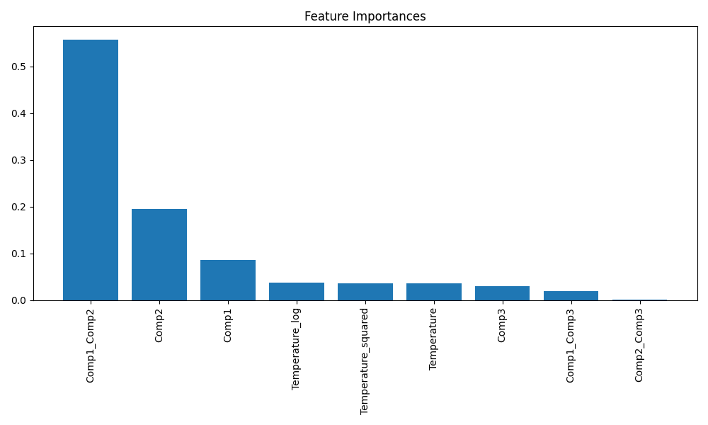
これらのグラフから、モデルの予測精度の高さと各特徴量の相対的な重要度を視覚的に確認できました。予測vs実際の値のプロットでは、点が対角線上にきれいに並んでおり、モデルの高い予測精度を示しています。特徴量重要度のバープロットからは、Comp1_Comp2の重要度が突出して高いことが一目でわかります。
4. まとめ
本実験では、Fortran による高速シミュレーションと Python の機械学習を組み合わせて、合金強度予測モデルを構築しました。具体的には以下のことを行いました:
Fortran を使用して、3元系合金の組成と温度に基づく強度計算シミュレーションを実装し、10,000 個のデータポイントを生成しました。
Python の scikit-learn ライブラリを用いて、生成されたデータに対してランダムフォレスト回帰モデルを構築しました。
元の特徴量に加えて、温度の2乗項、対数項、元素間の相互作用項などの新たな特徴量を追加し、モデルの性能向上を図りました。
その結果、以下のことが明らかになりました:
構築したモデルは高い予測精度を示し、テストデータに対する R2 スコアは 0.9973 となりました。
特徴量の重要度分析から、元素間の相互作用(特に Comp1_Comp2)が強度予測に最も大きな影響を与えていることがわかりました。
温度関連の特徴量も予測に一定の寄与をしていることが確認されました。
このアプローチにより、異なるプログラミング言語や技術を組み合わせることで、効率的なデータ生成と高精度な予測モデルの構築が可能であることが示されました。